Practical Mathematical Optimization

*This note is based on the book Practical mathematical optimization (Snyman et al., 2005).

Introduction

Formal Definition

Mathematical Optimization is the process of the formation and the solution of a constrained optimization problem of the general mathematical form:

\[\underset{w.r.t.\quad x}{minimize} f(x), x=[x_1, x_2, ..., x_n]^T \in \mathbb{R}^n\]

subject to the constraints:

\[g_j(x) \leq0, j=1, 2, ..., m\] \[h_j(x) = 0, j=1, 2, ..., m\]

where $ f(x), g_j(x) $ and $ h_j(x) $ are scalar functions of real column vector $ x $.

• (Design) Variables: The continuous components $x_i \in x $
• Objective Function: $ f(x) $
• Inequality Constraint Functions: $ g_j(x) $
• Equality Constraint Functions: $ h_j(x) $
• Optimal Vector: $ x^* $ and Optimal Function Value: $ f(x^*) $

Mathematical Optimization is often called Nonlinear Programming, Mathematical Programming, or Numerical Optimization.

4 Steps of Mathematical Modelling

1. The observation and study of the real-world situations associated with a practical problem.
2. The abstraction of the problem by the construction of a mathematical model
   • fixed model parameters $ p $
   • (design) variables $ x $

3. Find an analytical or numerical parameter-dependent solution $ x^(p) $. The problem to be solved in this step is, more often than not, a *mathematical optimization problem requiring a numerical solution.

4. Evaluation of $ x^*(p) $ and its practical implications

   • Adjustment of $ p $?
   • Refinement of the model?

Unconstrained 1-D Minimization

\[\underset{x}{minimize} f(x), x \in \mathbb{R}, f \in C^2\]

Newton-Raphson Method

Given an approximation $ x^0 $, iteratively compute:

\[x_{i+1} = x_i - \frac{f(x_i)}{f'(x_i)}\]

Hopefully, the iterations converge, i.e. $ \underset{i \rightarrow \infty}{lim} x_i = x^* $

Difficulties:

• The method is not always convergent, even if $ x_0 $ is close to $ x^* $
• The method requires the computation of $ H(x) $ at each step

Constraints

The boundary can be a line, surface, or hyper-surface.

Feasible region and Infeasible region.

Inequality Constrained:

\[\underset{x}{min} f(x), \\ such\ that\ g(x) \leq 0\]

Equality Constrained:

\[\underset{x}{min} f(x), \\ such\ that\ h(x) = 0\]

Linear Programming

When both the objective function and all the constraints are linear functions.

\[\underset{x}{min} f(x) = c^Tx, such\ that\ Ax \leq b; x \geq 0\]

where $ c $ is a real $ n \times 1 $ vector, b is a real $ m \times 1 $ vector and $ A $ is a $ m \times n $ matrix.

Convexity

A line through the points $ x_1 $ and $ x_2 $ is the set:

\[L = \{ x \ |\ x = x_1 + \lambda (x_2 - x_1),\ for\ all\ \lambda \in \mathbb{R}^n \}\]

A set $ X $ is a convex set if for all $ x^1, x^2 \in X $ it follows that

\[x = \lambda x_2 + (1 - \lambda) x_1 \in X,\ for\ all\ 0 \leq \lambda \leq 1\]

A function $ f(x) $ is a convex function over a convex set $ X $ if for all $ x_1, x_2 \in X $ and for all $ \lambda \in [0, 1] $:

\[f(\lambda x_2 + (1 - \lambda) x_1) \leq \lambda f(x_2) + (1 - \lambda) f(x_1)\]

The function is strictly convex if $ < $ applies.

Concave functions are similarly defined.

Gradient

For a function $ f(x) \in C^2 $ there exists a gradient vector at any point $ x $:

\[\nabla f(x) = \begin{bmatrix} \frac{\partial f}{\partial x_1} (x) \\ \frac{\partial f}{\partial x_2} (x) \\ \vdots \\ \frac{\partial f}{\partial x_n} (x) \\ \end{bmatrix}\]

If the function $ f(x) $ is smooth, then the gradient vector $ \nabla f(x) $ is always perpendicular to the contours in the direction of maximum increase.

Hessian Matrix

If $ f(x) $ is twice continuously differentiable ($ f(x) \in C^2 $) at point $ x $, there exists a matrix of second-order partial derivatives or Hessian matrix

\[\begin{aligned} H(x) & = \{ \frac{\partial^2f }{\partial x_i \partial x_j}(x) \} = \nabla^2f(x) \\ & = \begin{bmatrix} \frac{\partial^2 f}{\partial x_1^2} (x) & \frac{\partial^2 f}{\partial x_1 x_2}(x) & \dots & \frac{\partial^2 f}{\partial x_1 x_n}(x) \\ \frac{\partial^2 f}{\partial x_2 x_1} (x) & \frac{\partial^2 f}{\partial x_2^2} (x) & \dots & \vdots \\ \vdots & \vdots & \ddots & \vdots \\ \frac{\partial^2 f}{\partial x_n x_1} (x) & \dots & \dots & \frac{\partial^2 f}{\partial x_n^2} (x)\\ \end{bmatrix}_{n \times n} \end{aligned}\]

Test for Convexity

If $ f(x) \in C^2 $ is defined over a convex set $ X $, it can be shown that if $ H(x) $ is positive-definite for all $ x \in X $, then $ f(x) $ is strictly convex over $ X $.

Quadratic Function in $ \mathbb{R}^n $

The quadratic function in $ n $ variables can be written as:

\[f(x) = \frac{1}{2} x^TAx + b^Tx + c\]

where $ c \in \mathbb{R} $, b is a real $ n \times 1 $ vector and A is a $ n \times n $ real matrix that can be chosen in a non-unique manner. It’s typically chosen symmetrical which casts it as follows:

\[\begin{aligned} \nabla f(x) &= Ax + b \\ H(x) &= A \end{aligned}\]

• The function $ f(x) $ is called positive-definite if $ A $ is positive-definite
• The function $ f(x) $ is called convex if $ H(x) $ is positive-definite

Directional Derivative

The directional derivative of a scalar function $ f(x) $ with respect to a vector $ \vec{v} = \langle v_1, v_2 \rangle $ at a point $ x $ where $ |\vec{v}| = 1 $:

\[\nabla _v f(x) = \nabla^T f(x) v\]

Minima and Saddle Points

Global Minimum

$ x^* $ is the global minimum over the set if:

\[f(x) \geq f(x^*),\ for\ all\ x\in X \subset \mathbb{R}^n\]

Strong Local Minimum

$ x^* $ is a strong local minimum if there exists an $ \varepsilon > 0 $ such that:

\[f(x) > f(x^*),\ for\ all\ \{x \bigm| \vert\vert x-x^* \vert\vert < \varepsilon \}\]

The necessary and sufficient conditions:

1. $ f(x^*) = 0 $
2. $ H(x^*) $ is positive-definite
3. (Implicit) $ x^* $ is an unconstrained minimum interior to $ X $

If $ x^* $ lies on the boundary of $ X $, then: \(\nabla^Tf(x^*)\vec{v} \geq 0\) for all allowable directions $ \vec{v} $ such that $ x^* + \lambda \vec{v} \in X $ for $ \lambda > 0 $.

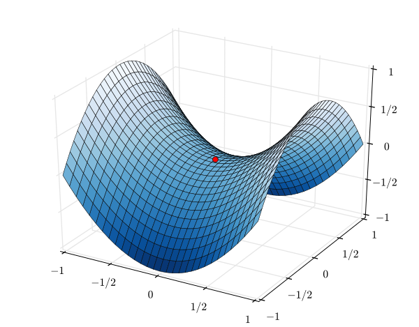
Saddle Points

A saddle point or minimax point is a point where the slopes (derivatives) in orthogonal directions are all zeros (a critical point), but not a local extremum.

Local Behavior of a Multi-variable Function

The truncated second-order Taylor expansion for a multi-variable function: \(f(x' + \delta) = f(x') + \nabla^T f(x') \delta + \frac{1}{2} \delta^TH(x' + \theta \delta)\delta\) for some $ \theta \in [0, 1] $

Line Search Descent Methods for Unconstrained Minimization

(Skipped Temporarily)

Standard Methods for Constrained Optimization

(Skipped Temporarily)

Basic Optimization Theorems

(Skipped Temporarily)

Appendix

Scalar Function

\(f: \mathbb{R}^n \rightarrow \mathbb{R}\) A scalar function is a function (of one or more variables) with a one-dimensional scalar output. It gives you a single value.

The codomain of the function is exactly the set of real numbers. An n-variable scalar function is a map from $ \mathbb{R}^n $ to the real number line $ \mathbb{R} $.

$ C^k $ Function

A function with $ k $ continuous derivatives on domain $ X $ is called a $ C^k(X) $ function.

Functions Evaluation

Analytical Formula

e.g. \(f(x) = x_1^2 + 2 x_2^2 + sin (x_3)\)

formulae: plural of formula

Computational Process

e.g. \(g_1(x) = a(x) - a_{max}\) where $ a(x) $ is the stress at some point in a structure (computed by means of a finite element analysis). The design is specified by $ x $.

Physical Process Measurements

e.g. \(h_1(x) = T(x) - T_0\) where $ T(x) $ is the temperature measured at some specified point in a reactor and $ x $ is the vector of operational settings.

Reference

---

1. Glasman-Deal, H. (2009). Science research writing for non-native speakers of English. World Scientific.
2. Snyman, J. A., Wilke, D. N., & others. (2005). Practical mathematical optimization. Springer.